How to lose 99.9% and still score a 500x

Crypto traders are insatiable. Listening to some of them, you would think that the crypto price action is getting boring. The price of ETH was 80 USD a bit more than a year ago and now it's 3000 USD, that was fun they say, but what's the remaining upside? 2x? 10x? 20x? Boring. They want more. Leverage? Too much hassle, requires constant management and could get liquidated.

Are you currently in the above mindset, or are you simply looking to considerably grow returns on your ETH holdings by taking more risk - as in, risk of complete anihilation of your position if you're wrong about long term price action? Or maybe you think it's all going to 0 and you want to magnify the returns of your leveraged short? If yes, or if you like some math in your finance, you might be interested in learning about constant leverage. This tool already exists in some forms in traditional financial markets, but can be made even more powerful thanks to the flexibility of decentralized, permissionless platforms. Yet, it seems it is not properly understood by some users in DeFi, especially from a quantitative point of view. This will be the subject of this blog post. Now the title may appear like clickbait, but constant leverage is an automated investment strategy that can actually lead to temporary ruin (-99.99%) while still eventually making x500 on the initial investment: quite the rollercoaster. Let's dive in!

What is constant leverage?

First let's recall with a simple example how leverage works. Assume that the price of ETH is currently 1000 USD. I deposit 10 ETH on Maker to get a collateralized loan of 5000 DAI. I buy more ETH with it and now have 15 ETH in a Maker vault. My debt-to-collateral ratio is 0.33 (33%), or equivalently I have a collateralization ratio of 3 (300%). A couple of weeks later, ETH has gone up to 2000 USD, which is a +100% gain. My 15 ETH are now worth 30K USD. I can sell a portion of debt to pay back my debt and be left with 25K USD, which is a +150% gain on my initial position. I made 1.5x more denominated in USD than I would have by just holding my original 10 ETH. We say that my position had a leverage ratio L of 1.5. It can be shown that the relationship between collateralization ratio R and leverage ratio is (only valid if all of the debt is used to buy ETH to add as collateral):

L = \frac{R}{R-1}

But we only compared the start and end point. Somewhere between 1K and 2K, say 1.5K, the 15 ETH collateral was worth 22.5K USD, which is in this example a collateralization ratio of 450% or a leverage ratio of ~1.3. So now between this price level and the end point, the return is only going to be increased by a factor of 1.3 compared to if I were to close my position. So to increase my overall return, one could do the following:

When the price reaches 1500 USD, generate more debt from my position, such that my collateralization ratio gets back down to 200%.
Buy more ETH with the newly generated DAI.
The position is now again at a leverage ratio of 1.5.

If that sounds familiar, that may be because this is exactly what the Boost feature of DeFi Saver does. By doing this periodically, one could significantly magnify returns. If the price goes down, one might want to protect themselves from liquidation by increasing their leverage ratio which corresponds to the liquidation protection mechanism of DeFi Saver or Instadapp. Assuming zero gas fees and zero slippage, one could even do either of these operations as soon as the price moves by just +/- 0.000001% to keep the same leverage ratio no matter what the price is, hence the term constant leverage which would be the continuous limit.

Similar arrangements exist both on centralized crypto exchanges in the form for example ETHBULL and ETHBEAR tokens on FTX, or on traditional markets where leveraged ETFs such as the TQQQ targeting a 3x increase in daily return. These are adjusted daily, which means that if the price moves a lot within the same day, one might miss out on some price action. In either cases, such a construct can significantly magnify returns, both positive and negative.

"Significantly" magnify, sure, but by how much? Let's take a look at some of the math behind constant leverage to figure this out.

A bit of math

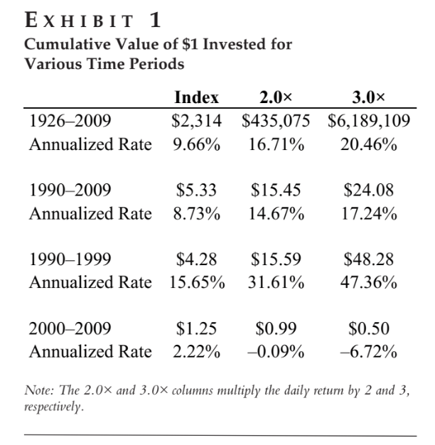
Before diving into the math, let's use an example to showcase the insane power of constant leverage both to build wealth or wreck complete havoc. In Trainor (2011), it is calculated that if a 3x leveraged ETF similar to the TQQQ had been used to bet on the stock market between 1926 and 2009 would have increased the total returns compared to just holding the non leveraged fund by a staggering 2675x, for a total return of 6,189,109x!!! However, this would have been at the cost of great ruin during the 1929 crisis with an almost complete annihilation of the portfolio and a -99.8% temporary loss -- but you have no idea that it will be temporary when it happens. This time period is of course unrealistic, but comfortable magnifications are observed for more realistic timeframes of 10 and 20 years as seen in the table below.

With these numbers, one might suspect that there's a power law at play somewhere, and they would be right! As it turns out, the continuous limit of doing constant leverage is equivalent to buying a synthetic that will track the power of the price of ETH. Specifically, if the price of ETH as a function of time is denoted $S_t$ , and the leverage ratio used is $L$ , the constant leverage portfolio value will move proportionally to $S_t^L$ under some standard assumptions. If you like DeFi mechanism design, this might remind you of the Power Perpetual primitive proposed by Paradigm and others, and indeed there might be some similarities in the underlying mathematical structure.

Avellaneda and Zhang (2010) derived the evolution of the constant leverage portfolio value in a specific case. Say the price of the underlying $S_t$ follows an Ito process, which is a generalization of a Geometric Brownian Motion (GBM):

\frac{d S_{t}}{S_{t}}=\sigma_{t} d W_{t}+\mu_{t} d t

Here $\sigma_{t}$ and $\mu_{t}$ are the "instantaneous" volatility and drifts, which means that we're not assuming these are constant and they change randomly every infinitesimal timestep.

With a leverage ratio $L$ and neglecting the interest rate to borrow some amount of numéraire, as well as any administrative cost for the constant leverage strategy, it is shown that:

\frac{L_{t}}{L_{0}}=\left(\frac{S_{t}}{S_{0}}\right)^{L} \exp \left\{\frac{\left(L-L^{2}\right)}{2} \int_{0}^{t} \sigma_{s}^{2} d s\right\}

Where $L_t$ denotes the value of the constant leverage portfolio at time $t$ and the term $\displaystyle \int_{0}^{t} \sigma_{s}^{2} d s$ is the realized variance over the time period studied. As we can see, when $|L| > 1$ , the term inside the exponential is negative, such that in particular:

\forall L > 1, \ \frac{L_{t}}{L_{0}} < \left(\frac{S_{t}}{S_{0}}\right)^{L}

The more chaotic the price movement was the further we get from the power law. Note that this is only valid in the case that the price follows an Ito process, which includes GBMs.

This means that even if the price at the end of the time period is for example 10x higher than it was at the beginning, the portfolio will actually have lost money anyway if the variance was too high! Similarly, to outperform the simple buy-and-hold strategy, the variance needs to be lower than some threshold.

One way to understand this is by looking at a simplified example of a round trip where the price starts at $S_{0}$ , moves to $S_{1} < S_{0}$ , and then goes back to the start, $S_{2} = S_{0}$ . When the price is down, we need to repay some of the debt by selling some collateral collateral to maintain the same collateralization ratio. Then the price goes back up, so we need to keep the leverage constant we need to "boost" our position by generating more debt and buying collateral with it. Great traders might have noticed the issue here: the net result of our actions boils down to: buy high, sell low! Surely not a great thing. This is what can lead to losing value even if the price goes up overall.

In summary, constant leverage portfolios can be thought of as yielding returns at a maximum similar to if one was holding an index tracking the price of the underlying to the power of the leverage ratio, with lower returns when the realized variance is higher over a time period. The returns can be negative, even when the price went up overall. The higher the leverage ratio, the more sensitive to variance (i.e. volatility) the instrument will be, and the higher the upside needed to have positive return, or outperform the buy and hold strategy. Everything that was discussed can also obviously be applied to shorting with constant leverage.

Constant leverage in DeFi

There are a number of products in DeFi that are exploring the design space of constant leverage. The first iteration was the non-custodial automation system of DeFi Saver (DFS). Originally intended to protect positions from liquidation by selling some of the collateral inside the position to repay the debt, it turns out that this system is essentially a custom constant leverage machine. The way it works is that you can select a target collateralization ratio as well as two thresholds. If the price of the asset goes down such that your collateralization ratio gets below the repay threshold, the "Repay" function is called to get back to the target, and if the price goes up above threshold, the "Boost" function is called. This is illustrated by the automation interface of DFS in the image below. For convenience, this strategy will be called "Threshold-based Constant Leverage" or TCL in the following.

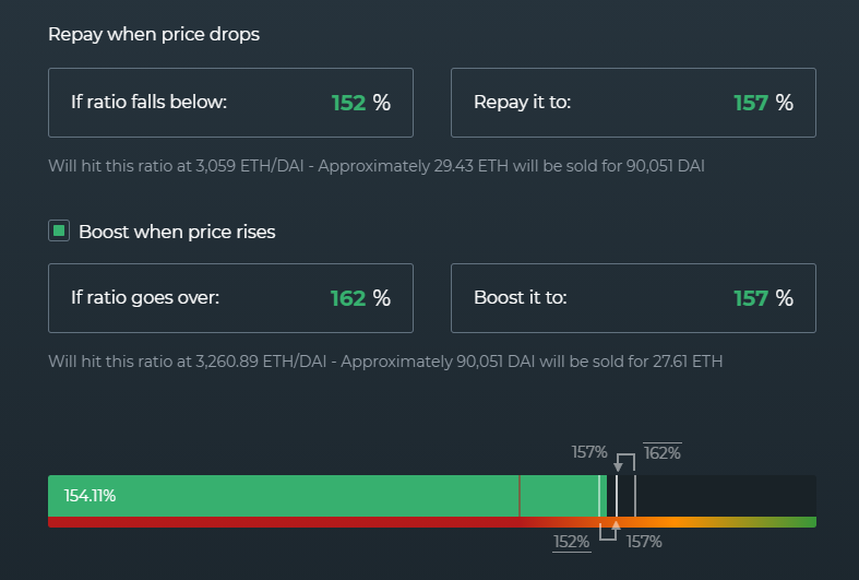
This is distinctly different from what exists in traditional finance in that the rebalances are price threshold based, instead of being based on time.

Other alternatives include the ETH 2x Flexible Leverage Index (ETH2X-FLI) token from the Index Coop, or the Cube tokens from Charm. Both have the distinct advantage of being decentralized, as opposed to DFS which is maintained by a centralized keeper bot - though it should be emphasized that it is still non-custodial and the bot cannot do anything else than rebalance when a condition is met.

None of these can perfectly replicate the continuous limit of constant leverage because the thresholds can be quite far from the target ratio. For example in the case of ETH2X-FLI, the leverage ratio might be anywhere between 1.7x and 2.3x as opposed to the target of 2x. For Cube tokens, it can move between 1.5x and 4x! As we will see, small differences can have an outsized effect on overall returns because of the power law that we uncovered previously.

In the case of DFS, while it would be theoretically possible to narrow the range to +/- 0.5%, the gas costs would essentially destroy the portfolio for small positions. However, these thresholds can be interesting to approximate constant leverage very closely.

In fact, it was shown by user mdmkolbe#3444 on Discord that a threshold based rebalancing protocol like DFS automation are identical to constant leverage when there are only boosts, or only repays, except that the effective leverage ratio of a TCL strategy will be slightly below or above the target ratio respectively. The difference is that in the continuous case, any tiny drawdown would eat into the portfolio value, whereas with the thresholds as long as the correction doesn't hit the repay threshold, there is no loss. Of course there is a catch: the effective constant leverage ratio might be lower when it the price goes up, and higher when the price goes down, which essentially makes things worse on that side. mdmkolbe#3444 showed for example that in the case when there are only boosts, the effective leverage ratio of the automated boosting strategy is:

L_{\mathrm{eff}} = \frac{\ln \left( \frac{B_f - 1}{B_t - 1} \right)}{\ln \left( \frac{B_f}{B_t} \right)}

Where $B_t$ and $B_f$ are the collateralization ratios to boost from and boost to respectively. This turns out to be lower than in the continous case. The same result applies in the repay case.

Simulating Threshold-based Constant Leverage (TCL)

To illustrate the different topics discussed here, I implemented a Python simulator of the DFS automation system because it is extremely flexible and can easily be used to model the continuous limit by choosing a small interval. The full code as well as explanations on on how to use it are available on GitHub. Now it's time to dive into some concrete results, and most importantly to show that my title wasn't as clickbait as it seems!

The set up of the simulations is as follows: a TCL vault is created with settings $R_f, \ R_t, \ B_f, \ B_t$ which are the thresholds to repay from, the target to repay to, boost from and boost to respectively. Annualized volatility and drift are then prescribed to generate a number of geometric brownian motion paths for the price of the collateral. For each path, we obtain the final return of the position, which allows us to extract a probability distribution of returns and make observations such as the probability of profit of a given strategy or the probability of outperforming the average market trend.

All results are presented with averages over 1000 random paths. For those unfamiliar, the annualized drift expresses the expected log growth of the asset over a year in a probabilistic sense. For example, if the asset has an expected growth of 10x in a year, this means that running $N \rightarrow \infty$ simulations should yield an average terminal price 10x above the initial price, corresponding to a drift of $\ln(10) \simeq 2.3$ .

We can first try to approach the continuous case as close as possible assuming no gas fee and no service fee for the automation and boost operations. Since rebalances are threshold based, this means that we need to have almost continuous time, and thresholds at an very close to the target.

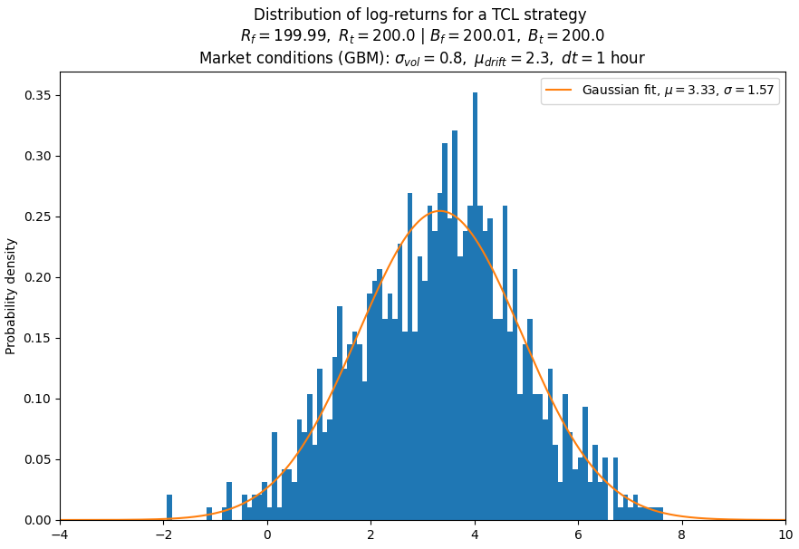
In these assumed market conditions of a 10x expected yearly growth in a 80% volatility environment, we see that the expected log-return of this 2x TCL (remember that the leverage ratio is given by $\frac{R}{R-1}$ where $R$ is the target collateralization ratio) is 3.33, or an actual return of 28x which is overperforming the market by 2.8x, better than the leverage ratio. This is only the mean return though, and we can see that this distribution is quite wide. Integrating we find that there is a 10% chance of outperforming the average market growth by a factor of 10 for a total return of 200x. If all we're interested in is USD gains, the probability of being in profit not minding an underperformance rounds to a 98% chance. Sounds too good to be true? You're right to be skeptical. Let's see what happens if the expected growth is "only" 2x with the same volatility.

Things don't look so good anymore. Now the average return is just 1x and the probability of profit is barely above flipping a coin. There is a 65% chance that this strategy will underperform, and a significant chance of ending up with a -50% loss or more despite the market going 2x.

What we see with these two simple examples is the illustration of what we discussed in the first paragraph: there is a fundamental relationship between growth and volatility leading to a TCL strategy being extremely profitable, or ruinous. The growth of the underlying asset needs to be large enough to compensate for the volatility losses along the way. And there's more. We only looked at the overall returns here, but even in the case of a strategy that ends up outperforming the market on a given realized price path, it might have suffered a massive transient loss upwards to 99.9%. That's how powerful constant leverage is in both directions, it can make you temporarily ruined while still growing so much that you recover if the market grows enough, or temporarily extremely rich while still being able to ruin you. On the other hand, if a trader implementing a constant leverage strategy is wrong about the kind of realized volatility that can be expected between two price points, they might be in for a rude awakening.

Let's look at a more practical example now and have some fun. Let's say DeFi Saver is deployed on a cheap layer 2, making gas prices low enough that a +/- 5% threshold would make sense for a variety of initial positions. Let's further assume that it's possible to go as low as 135% collateralization before liquidation, making a 145 - 150 | 150 - 155 setting sensible: this corresponds to a constant leverage of ~3x. We'll look at a collateral asset that we expect to grow 20x within a year, with a volatility of 110%. Somewhat of a realistic expectation for crypto assets. If you hate cryptocurrencies and think they're going to zero, you can just imagine that we're simulating a short all the way down to a >99% loss under the same volatility.

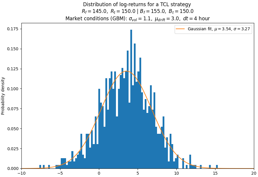
We obtain a ~85% chance of being in profit under these conditions, although there is a ~45% chance that we'll underperform the market. However, there is ~15% chance that we'll outperfom the market by a factor of 50x for an overall return of 1000x, with a maximum temporary loss over the 1000 runs of... 99.9999%! Or How to lose 100% and still make a 1000x. See, my title could have been even more clickbaity :)

Conclusion

Constant leverage exists in traditional finance but incurs relatively large management costs and lack flexibility, being limited to daily rebalances. An open infrastructure like that of DeFi platforms can make it more transparent, more efficient, and allow to approach the theoretical payoff of the coninous limit much closer. This also makes the product significantly more powerful both ways, leading to incredible returns or ruin. Even though a number of assumptions were made here (0 interest rate for borrowing, zero management cost), I hope that this blog post shed light on some of the quantitative characteristics of this financial product and how it can be implemented in DeFi. Don't hesitate to play with the simulator or suggest some changes to improve it.